import numpy as np
import matplotlib.pyplot as plt
import pandas as pd

plt.style.use("ggplot")Ornstein-Uhlenbeck Process
The famous Ornstein-Uhlenbeck Process takes the form \[ d x_t=\theta\left(\mu-x_t\right) d t+\sigma d W_t \] which is a stationary process in contrast to Wiener process. \(\mu\) represents the equilibrium value, \(\theta\) is the rate of reverting to equilibrium.
This process can be used for modeling interest rate and FX rate in pair trading strategy, which is making use of mean reversion feature of certain assets.
def gen_OU_process(dt=0.1, theta=1.2, mu=0.5, sigma=0.3, n=1000):
    x = np.zeros(n)  # initiate the series
    for t in range(1, n):
        x[t] = (
            x[t - 1]
            + theta * (mu - x[t - 1]) * dt
            + sigma * np.random.normal(0, np.sqrt(dt))
        )
    return x


def plot_process(x):
    fig, ax = plt.subplots(figsize=(12, 6))
    ax.plot(x)
    ax.set_xlabel("t")
    ax.set_ylabel("x(t)")
    ax.set_title("Ornstein-Uhlenbeck Process")
    plt.show()


if __name__ == "__main__":
    x = gen_OU_process(mu=3)
    plot_process(x)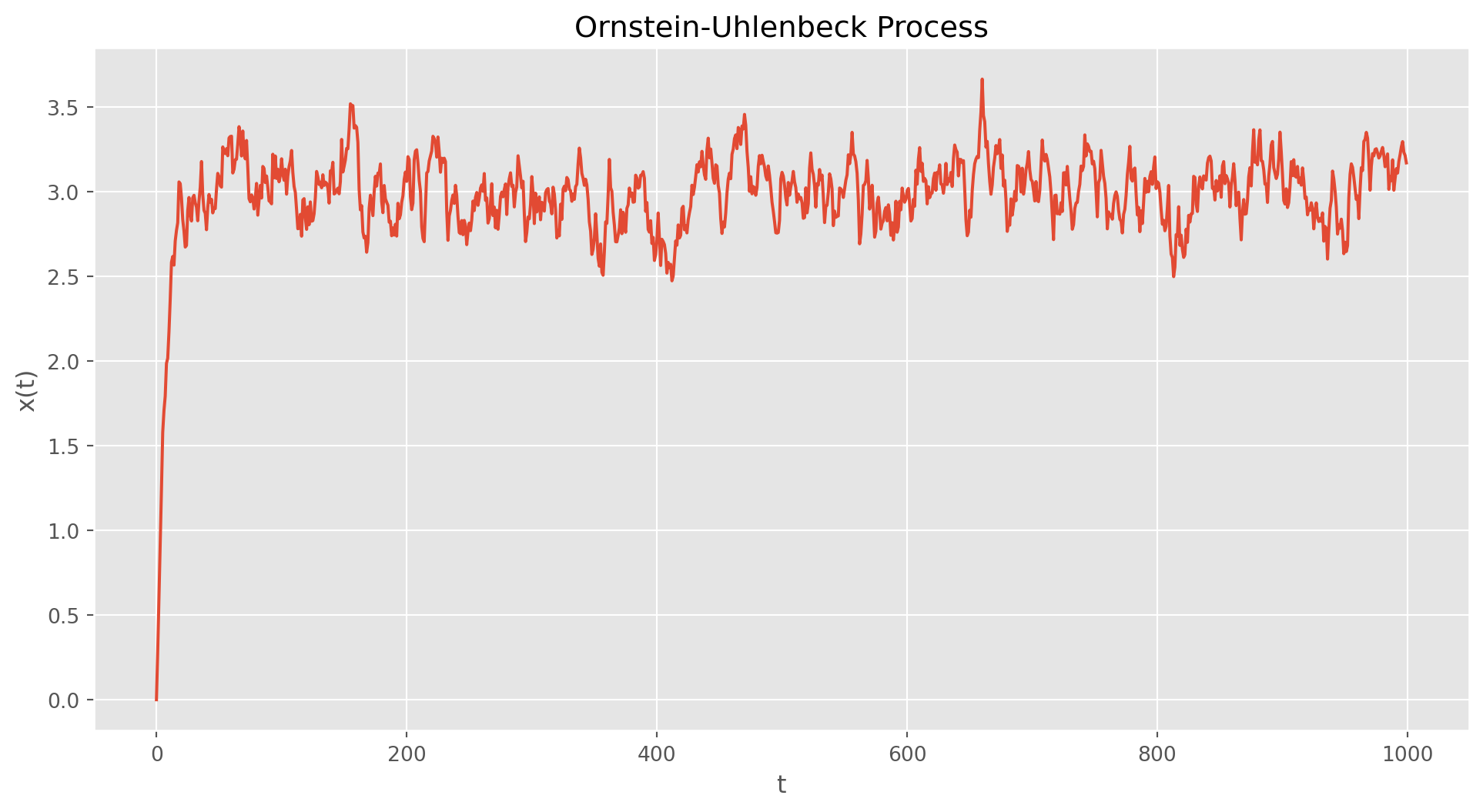
Vasicek Model
The model is named after Czech mathematician Oldřich Vašíček, which assumes that short term interest rate \(r(t)\) follows a mean-reverting Ornstein-Uhlenbeck Process. \[ dr(t) = \kappa (\theta-r(t))dt +\sigma d W(t) \] where \(dr(t)\) is the change of \(r(t)\), \(\kappa\) is the speed of mean reversion, other parameters the same as in Ornstein-Uhlenbeck Process. Note that this model allows negative interest rate.
def vasicek_model(r0, kappa, theta, sigma, T=1, N=1000):
    dt = T / N
    t = np.linspace(0, T, N + 1)
    rates = [r0]

    for i in range(N):
        dr = kappa * (theta - rates[-1]) * dt + sigma * np.random.normal(0, np.sqrt(dt))
        rates.append(rates[-1] + dr)

    return t, rates


def plot_process(t, r):
    fig, ax = plt.subplots(figsize=(12, 6))
    ax.plot(t, r)
    ax.set_xlabel("t")
    ax.set_ylabel("r")
    ax.set_title("Vasicek Model")
    plt.show()


if __name__ == "__main__":
    t, rates = vasicek_model(1.5, 0.01, 1.5, 0.1)
    plot_process(t, rates)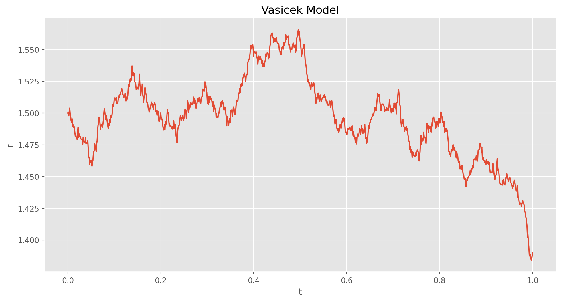
Bond Valuation with Vasicek Model
As a reminder, this is the continuous compounding formula assuming a constant \(r\) \[ P(t) = P_0 e^{rt} \]
If \(r(t)\) is a continuous stochastic process, then present value of an asset can be presented by \[ P_0 = P(t)\exp{\left(-\int_t^Tr(s)ds\right)} \]
num_of_simu = 1000
num_of_points = 200


def mc_vasicek_bonds(P, r0, kappa, theta, sigma, T=1):
    # P: principal of bond, T=1 one year
    dt = T / num_of_points
    results = []

    for i in range(num_of_simu):
        rates = [r0]
        for j in range(num_of_points):
            dr = kappa * (theta - rates[-1]) * dt + sigma * np.random.normal(
                0, np.sqrt(dt)
            )
            rates.append(rates[-1] + dr)
        results.append(rates)
    simu_data = pd.DataFrame(results).T

    integral_sum = simu_data.sum() * dt
    pv_integral_sum = np.exp(-integral_sum)
    bond_price = P * np.mean(pv_integral_sum)
    print("bond price based on MC: {}".format(bond_price))

    return simu_data


def plot_process(simu_data):
    fig, ax = plt.subplots(figsize=(12, 6))
    ax.plot(simu_data)
    # ax.set_xlabel('t')
    # ax.set_ylabel('r')
    ax.set_title("Bond yield MC Simulation")
    plt.show()


if __name__ == "__main__":
    simu_data = mc_vasicek_bonds(
        P=1000, r0=0.05, kappa=0.3, theta=-0.03, sigma=0.03, T=3
    )
    plot_process(simu_data)
bond price based on MC: 933.5834182265432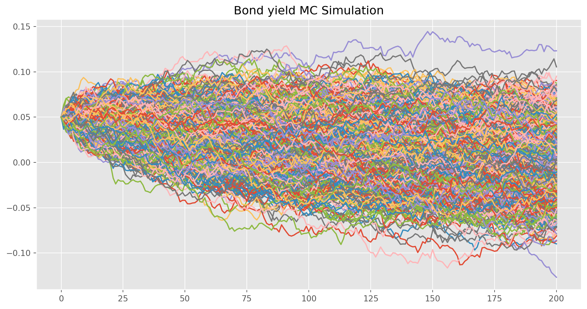
The solution of Stochastic Differential Equations (SDE) is a probability density function, however very few has closed-form solution.
Refresh of Ordinary Differential Equations
There are four types solution methods of Ordinary Differential Equation (ODE): separable equations, homogeneous method, integration factor and exact differential equations.
Separable Equations
Usual form \[ \frac{d y}{d x}=P(x) Q(y) \]
\[ \begin{align} \frac{dy}{dx} +2xy &= x\\ \int^y\frac{1}{1-2y} dy &= \int^x x dx\\ -\frac{1}{2}\ln{|1-2y|}&=\frac{1}{2}x^2+C \end{align} \] Then isolate \(y\), which gives us a closed-form solution.
Homogeneous Method
The homogeneous form ODE can be check by using \[ f(kx, ky) = f(x, y) \]
\[ \frac{d y}{d x}=\frac{x^2+y^2}{x y} \]
\[ \frac{d y}{d x}=\frac{\frac{x^2}{x^2}+\frac{y^2}{x^2}}{\frac{x y}{x^2}} \rightarrow \frac{d y}{d x}=\frac{1+\left(\frac{y}{x}\right)^2}{\frac{y}{x}} \]
Replace \(v=\frac{y}{x}\)
\[ \begin{aligned} & \frac{\partial y}{\partial x}=\frac{1+v^2}{v} \\ & x \frac{\partial v}{\partial x}+v=\frac{1+v^2}{v}\\ & x \frac{\partial v}{\partial x}+v=\frac{1}{v}+{v} \end{aligned} \]
\[ \begin{aligned} & \int v d v=\int \frac{1}{x} d x \\ & \frac{1}{2} v^2=\ln |x|+c \\ & v^2=2 \ln |x|+c \\ & v=\pm \sqrt{2 \ln |x|+c}\\ & y = \pm x \sqrt{2 \ln|x|+c} \end{aligned} \]
Stochastic Differential Equations
\[ \text{SDE=ODE + GWN} \] where \(\text{GWN}\) stands for Gaussian White Noise.
The Brownian motion , sometimes also know as Wiener process, is a fractal in nature, the function will not be differentiable with a well-defined gradient. A standard Brownian motion has following characteristics
\[ \begin{aligned} W(0) & =0 \text { a.s. } \\ E[W(t)] & =0(\mu=0) \\ E\left[W^2(t)\right] & =t\left(\sigma^2=1\right) \end{aligned} \]
However, due to fractal nature \[ \frac{W_t}{t} \] does not exist.